Ultrasonic Technology
Ultrasound
Ultrasound is the oscillating sound wave above human hearing range (20 Hz – 20 kHz and is typically defined from 20 kHz up to Megahertz range. It has a wide range of applications in disciplines such as chemistry, physics, biology, engineering, oceanography, food industry, medicine and seismology. Examples of such applications include SAW (Surface Acoustic Waves) signal-processing devices in analogue signal processing, medical applications such as fetal, cardiac, urological and ophthalmological imaging using noninvasive acoustics and cleaning heavily contaminated devices with complicated surface structure such as greased machine components and soiled surgical instruments. Our project will focus on the cleaning property of the ultrasound. The underlying physics behind ultrasound cleaning is liquid cavitation, explained below.
Ultrasonic frequencies are produced in the liquid-filled tank by transducers such as piezoelectric ceramic and magnetostrictive attached to the tank. However, magnetostrictive transducers are not used at frequencies above 30 kHz because controlling the motion and vibration of large mass of materials involved in these transducers can get harder beyond 30 kHz. As UltraClean operates beyond 30 kHz [Appendix A, Table 1] for lighter loads such as surgical apparatus, piezoelectric transducer is chosen. When a piezoelectric material is induced an electric current, they change in size and hence vibrate the diaphragm attached to it. When electric current is repeatedly applied to it, the diaphragm moves forward and backward in one direction. When this is attached to the liquid-filled cleaning tank, the ultrasonic wave at the frequency of vibrating diaphragm propagates through the liquid, compresses and decompresses, and hence produces cavitation bubbles of high energy [Appendix A, Diagram 1, Diagram 2].
Cavitation Bubble Dynamics
When those bubbles collapse, they generate temperature of several thousand kelvin and shoot out the high pressure liquid jet, effectively removing soil and debris away from the surface and hard-to-reach crevices. The underlying physics behind liquid cavitation is calculated and explained more in Appendix A, Section 7. The Blake threshold pressure (pB) at which the bubble explodes can be calculated as where p0 is the hydrostatic pressure, 𝜎 is the surface tension of the liquid and R0 is the radius of the cavitation bubble. For example, the rupture and the overshoot of the bubble at ultrasonic resonant frequency of 20 kHz can be found in Appendix A, Figure 6.
MBSL (Multi-Bubble Sonoluminescence) emission temperature (T) can be quantitatively determined in Suslick and Flannigan’s emission line intensity equation where h is Planck’s constant, c is the speed of light, k is Boltzmann’s constant, l is the path length of confining region, 𝜌0 is the atom number density, gn is the degeneracy of the upper state, Q is the partition function and Anm is Einstein transition probability between states n and m [1, Page 195]. The force by the bubble collapse can be described by for large bubbles and for small bubbles [8, Page 190] where x is the bubble’s position in a standing wave field, 𝜀0 is free space permittivity, is the applied acoustic pressure and V0 is the bubble volume. The volume of the cavitation bubble can be determined as where V0 () is the equilibrium volume. As can be seen, the resonant frequency of the transducer determines the size and the magnitude of the resonant bubbles.
Low ultrasonic frequencies create fewer cavitation bubble implosions with higher energy release whilst higher frequencies create more cavitation bubble implosions with lower energy release within a given time. Choice of frequency and related cavitation bubble size is important depending on type of parts to be cleaned: 25 kHz for heavy parts and big tanks, 40 kHz for 95% of most applications, 68 kHz for buffed soft metal components, 132 kHz for disk drive components and 170 kHz for disk drives in semiconductor industry [9].
Ultrasonic Wave Generation
To create the high frequency waves we used a 555 chip in “astable” mode. In this mode the output of the chip is a square wave with frequency and duty cycle dependant on capacitor and resistor values. We can understand this mode by looking at one other mode of the 555, the “monostable” mode. This mode uses a negative slope as a trigger, which starts the charging of a capacitor and the output goes high. When the voltage on the capacitor reaches 2/3 of VCC, the output goes low. In the “astable” mode the trigger is connected to the output, so it triggers itself, creating a square wave.
The frequency of this wave is determined by: [20]
From the datasheet it recommends that for 40kHz, , and duty cycle is , due to this we soon realised that to get at duty cycle of 50% Ra would have to be 0Ohms, therefore to obtain this would be impossible. We therefore settled with C=1nF, Ra=1kOhm and Rb=18kOhm. This theoretically gives a frequency of 39kHz and duty cycle of 51.35%. However when testing this in PSpice, this resulted in a frequency of 40.98kHz. This could be due to changes in temperature causing effects on the capacitor. Therefore, we may have to change these values again, to get more robust frequency, due to conditions in the country of use. The wave generated [Appendix A, Diagram 4] can be further amplified according to the ultrasonic tank size and the load. Figure 1 shows a sample wave generation circuit which produces ~40 kHz square waves.
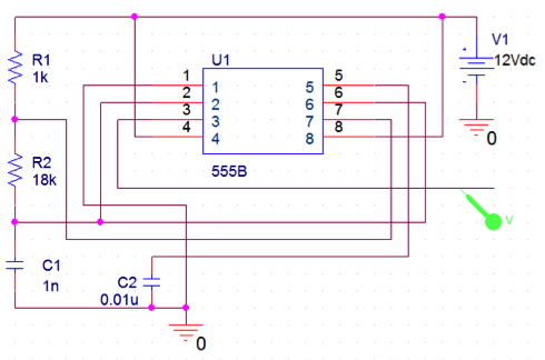
Figure 1: Sample 40 kHz square wave generator circuit to connect to piezoelectric transducer after amplification (PSpice)